The Euro 2024 ⚽ is a nice showcase of Bayesian Statistics. In Bayesian statistics, probabilities are seen as a degree of belief, which fits well with the nature of football. Almost everyone has beliefs about the strengths and weaknesses of the teams before seeing any games (based on historical data) and then updates these beliefs as new data comes in (games have been played).
#Some R-Magic to convert the team names to numbers, no need to understand thisng =nrow(data)teams =unique(data$Home)nt =length(teams)ht =unlist(sapply(1:ng, function(g) which(teams == data$Home[g])))at =unlist(sapply(1:ng, function(g) which(teams == data$Away[g])))np=1#Number games leaving out for predictionngob = ng-np #ngames obsered ngob = number of games to fit#print(paste0("Using the first ", ngob, " games to fit the model and ", np, " games to predict.", "Num teams ", length(teams)))my_data =list(nt = nt, ng = ngob,ht = ht[1:ngob], at = at[1:ngob], s1 = data$score1[1:ngob],s2 = data$score2[1:ngob],np = np,htnew = ht[(ngob+1):ng],atnew = at[(ngob+1):ng],s1new = data$score1[(ngob+1):ng],s2new = data$score2[(ngob+1):ng])
Using the first 115 games to fit the model and 1 games to predict. In total we have 24 teams.
A Model for the goals scored 🥅
We will assume that the number of goals scored by the home team \(s_1\) and the away team \(s_2\) follows a Poisson distribution. This has been shown to be a good model for the number of goals scored in a football match. We model the rate parameter \(\theta\) of the Poisson distribution, related to the attack and defense strengths of the teams, as follows:
\[
s_1 \sim \text{Pois}(\theta_1) \quad\text{goals scored by the home team}
\]
\[
s_2 \sim \text{Pois}(\theta_2) \quad\text{goals scored by the away team}
\]
This is equivalent to performing two separate Poisson regressions, one for each team.
Since there is no home advantage in the Euro (except for Germany), we set \(\text{home} = 0\).
Prior for the attack and defence strength
In Bayesian statistics, we further need to specify a prior for the parameters (our degree of believe in the attack and defense abilities before seeing any data). For that we use a hierarchical model with correlated parameters. Other models are investigated at comp_premier_league for the English Premier League 2019/2020 season and for the German Bundesliga 2000 and 2024 where the hierarchical model have been especially successful. The model is adopted from the blog_post and the paper. We extend the model to include a correlation between the attack and defense strength of the teams, since it is quite reasonable that a team that scores many goals (is above average in offense) is also good in defense.
Conditioning on the data / Fitting the model
After we state the model we fit the model to the data, or in Bayesian parlance, we update our degree of belief after seeing the data.
Details of the model MCMC sampling with Stan
The model is written in the probabilistic programming language Stan and can be found at https://github.com/oduerr/da/blob/master/website/Euro24/hier_model_cor.stan. This model used a Cholesky decomposition to model the correlation between the attack and defense strength of the teams. While this produces very effective sampling and is numerically stable, the Cholesky decomposition adds another layer of complexity to the model. We also provide a model without the Cholesky decomposition at https://github.com/oduerr/da/blob/master/website/Euro24/hier_model_cor_nocholesky.stan which is easier to understand but which is, besides the numerical difficulties, equivalent to the model with the Cholesky decomposition.
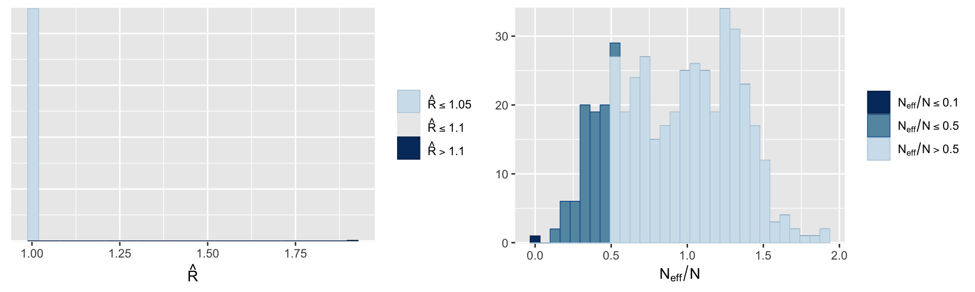
The fitting of the model is good, as the Rhat values are close to 1 and we have no divergent transitions. The effective sample size is also good.
The fitted model
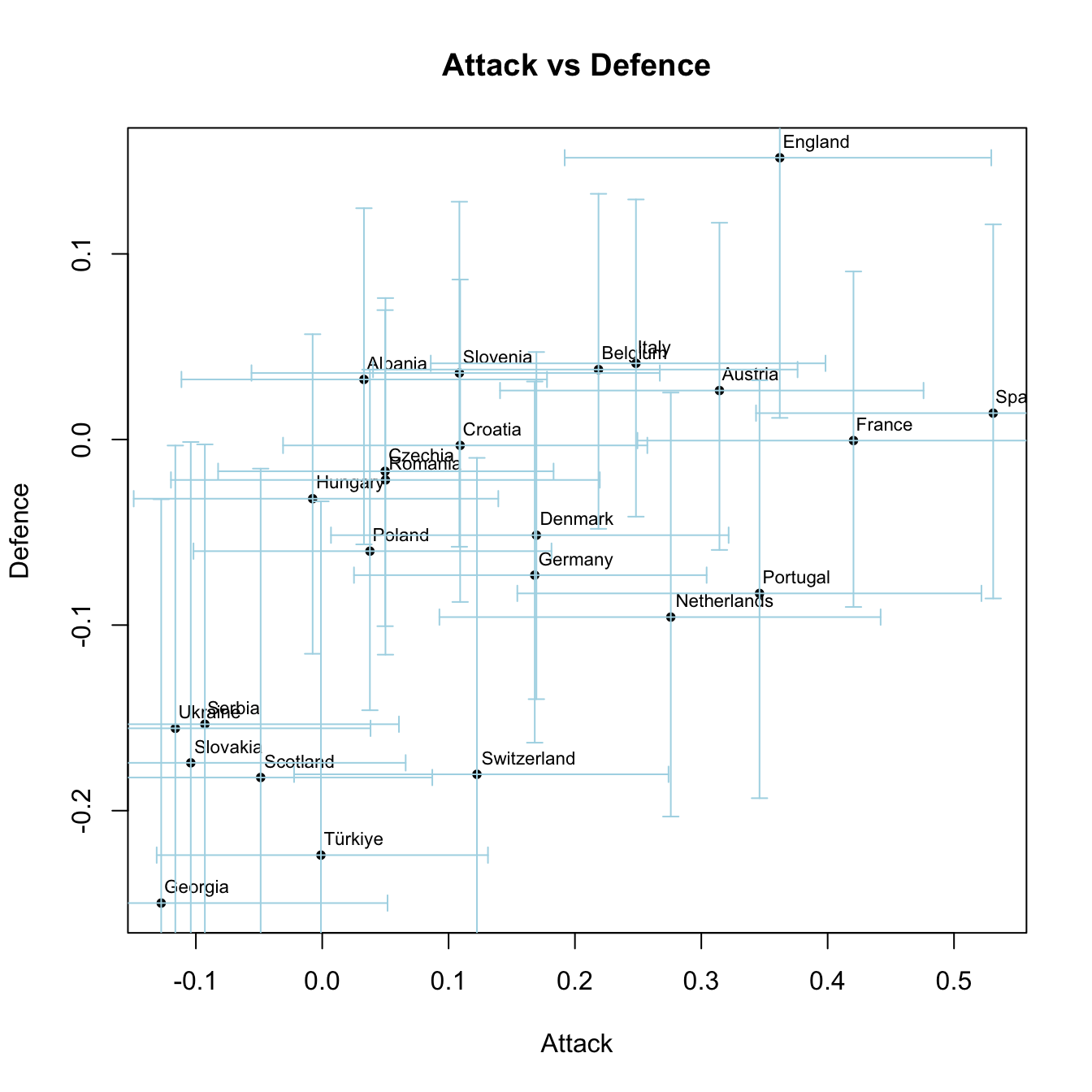
We plot the means of the attack and defense strengths of the teams. Shown are the mean values along with the 25% and 75% quantiles. There is considerable uncertainty in the strengths of the teams, but that’s the nature of the game.
Code
library(tidyverse)library(tidybayes)# Step 1: Gather draws and calculate summary statistics with credible intervalsd = hfit %>% tidybayes::gather_draws(A[i, j]) %>%group_by(i, j) %>%summarise(average_value =mean(.value),lower =quantile(.value, 0.25), # Lower bound upper =quantile(.value, 0.75), # Upper bound .groups ="drop" )# Step 2: Create a matrix of the average valuesA =xtabs(average_value ~ i + j, data = d)# Step 3: Plot the average valuesplot(A[1,], A[2,], pch=20, xlab='Attack', ylab='Defence', main='Attack vs Defence')# Step 4: Add team labelstext(A[1,], A[2,], labels=teams, cex=0.7, adj=c(-0.05, -0.8))# Step 5: Add error bars for 66% credibility intervals# Reshape data for plottingd_wide <- d %>%spread(key = j, value = average_value)d_lower <- d %>%spread(key = j, value = lower)d_upper <- d %>%spread(key = j, value = upper)# Convert to matrices for easier plottingA_lower <-xtabs(lower ~ i + j, data = d)A_upper <-xtabs(upper ~ i + j, data = d)# Plot vertical error barsarrows(A[1,], A_lower[2,], A[1,], A_upper[2,], angle=90, code=3, length=0.05, col="lightblue", alpha=0.5)# Plot horizontal error barsarrows(A_lower[1,], A[2,], A_upper[1,], A[2,], angle=90, code=3, length=0.05, col="lightblue")
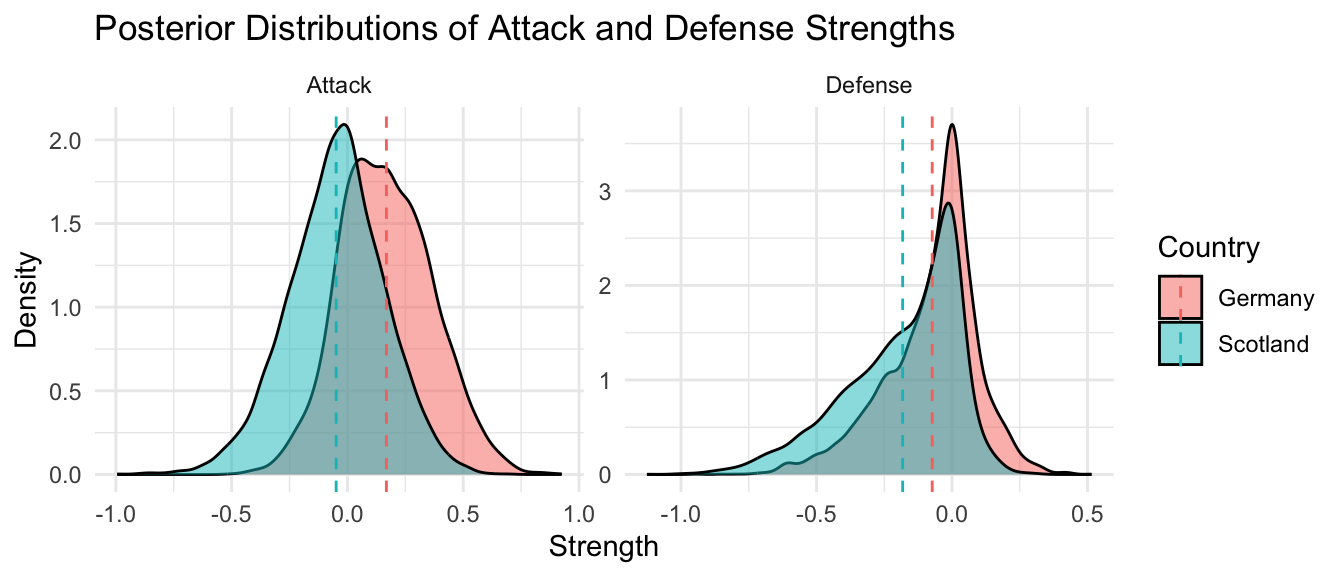
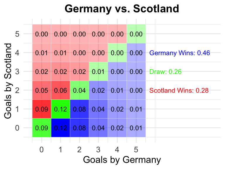
Detailed explanations for a single match Germany vs Scotland
The opening game of Euro 2024 was Germany vs. Scotland. In the plots below, we show the posterior probabilities for the attack and defense strengths of the teams.
Code
library(dplyr)library(tidyr)library(ggplot2)library(tidybayes)# Function to calculate probabilities for a pairingid1 <-which(teams =='Germany')id2 <-which(teams =='Scotland')# Extract posterior distributions for Attack and Defenseattack_germany <- hfit %>% tidybayes::spread_draws(A[i, j]) %>%filter(j == id1, i ==1) %>%select(A)attack_scotland <- hfit %>% tidybayes::spread_draws(A[i, j]) %>%filter(j == id2, i ==1) %>%select(A)defense_germany <- hfit %>% tidybayes::spread_draws(A[i, j]) %>%filter(j == id1, i ==2) %>%select(A)defense_scotland <- hfit %>% tidybayes::spread_draws(A[i, j]) %>%filter(j == id2, i ==2) %>%select(A)# Combine data into a tidy data frametidy_df <-bind_rows( attack_germany %>%mutate(Statistic ="Attack", Country ="Germany"), attack_scotland %>%mutate(Statistic ="Attack", Country ="Scotland"), defense_germany %>%mutate(Statistic ="Defense", Country ="Germany"), defense_scotland %>%mutate(Statistic ="Defense", Country ="Scotland"))# Include the mean values in the plotggplot(tidy_df, aes(x = A, fill = Country)) +geom_density(alpha =0.5) +facet_wrap(~ Statistic, scales ="free") +labs(title ="Posterior Distributions of Attack and Defense Strengths", x ="Strength", y ="Density") +geom_vline(data = tidy_df %>%group_by(Statistic, Country) %>%summarise(mean_A =mean(A)), aes(xintercept = mean_A, color = Country), linetype ="dashed") +theme_minimal()
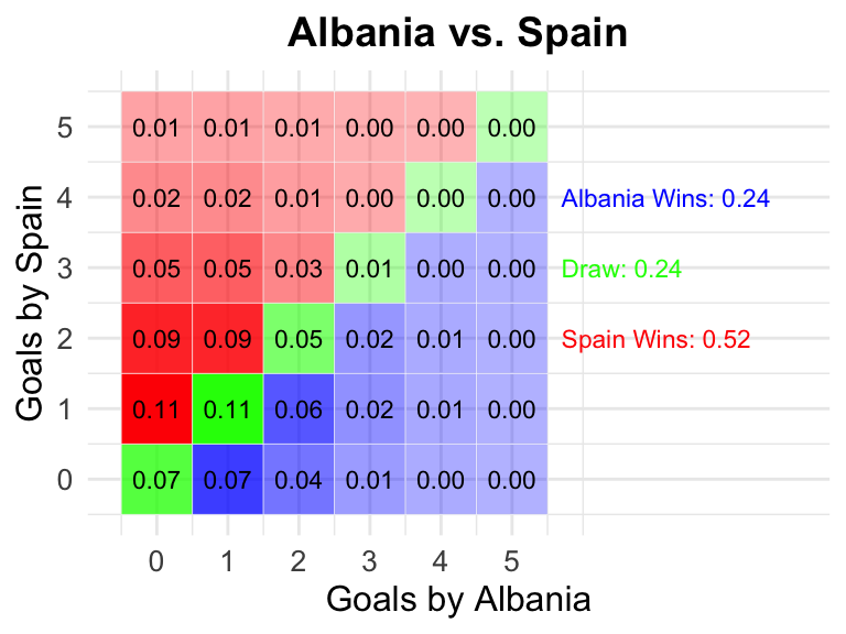
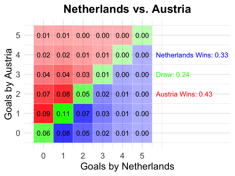
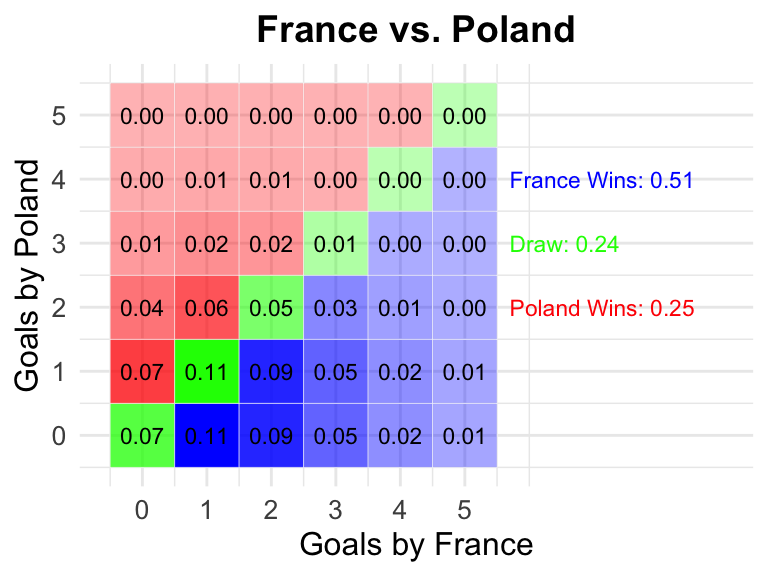
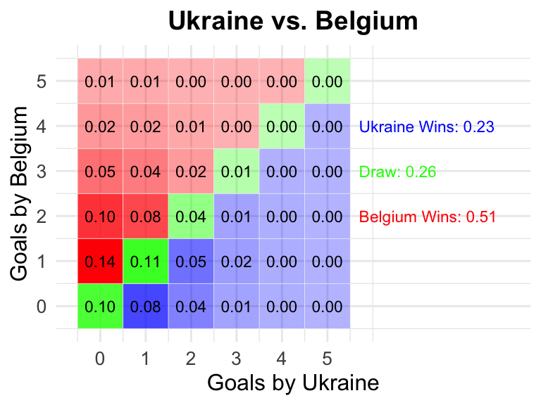
Making predictions
We can now make predictions for the game Germany vs Scotland. Below are the first samples of the posterior distribution for the attack and defense strengths of germany and scotland.
Code
# Extract first five samples for demonstrationdf =data.frame(attack_germany = attack_germany$A, defense_germany = defense_germany$A, attack_scotland = attack_scotland$A, defense_scotland = defense_scotland$A) %>%head() knitr::kable(df)
attack_germany
defense_germany
attack_scotland
defense_scotland
-0.0442763
-0.0242716
0.1630760
-0.1346680
0.3273970
-0.0198311
-0.0108560
0.0377780
0.2607110
-0.1016880
-0.2155270
-0.4300470
-0.0570626
-0.0008690
0.0580947
0.0156115
0.0885649
0.0009105
0.1246280
0.0193857
0.4273620
-0.0032764
0.1563150
0.0513863
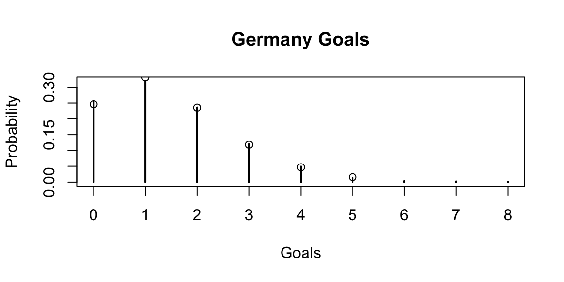
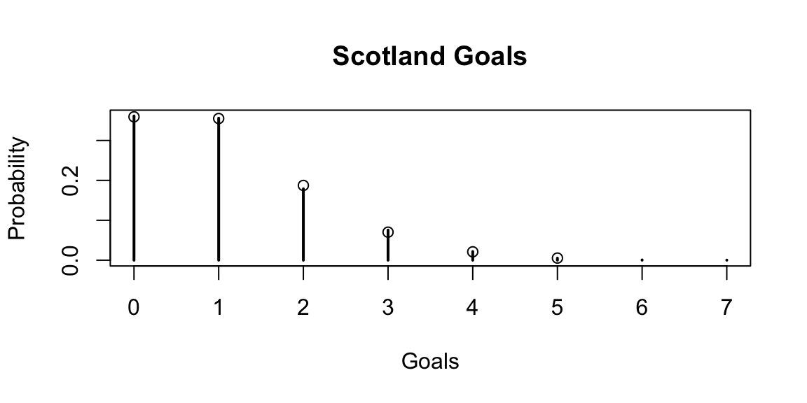
We use the samples for posterior row by row to sample the number of goals for Germany and Scotland. We can use the samples to calculate the probability of a win, draw or loss for Germany.
Probabilities for win/draw/loss
Code
set.seed(42) theta_germany =exp(attack_germany$A - defense_scotland$A) theta_scotland =exp(attack_scotland$A - defense_germany$A) g_germany =rpois(length(theta_germany), theta_germany) g_scotland =rpois(length(theta_scotland), theta_scotland)# Alternative way to calculate the probabilities calc_prob <-function(observed, theta) {mean(dpois(observed, theta)) }plot(table(g_germany)/length(g_germany), main='Germany Goals', xlab='Goals', ylab='Probability') prob_goals_germany =apply(matrix(0:10, ncol=1), 1, function(x) calc_prob(x, theta_germany))points(0:5, prob_goals_germany[1:6])
Another way to look at is is at the joint distribution of the goals scored
Code
library(tidyverse)library(ggplot2)# Define the functionplot_goal_probabilities <-function(attack_team1, defense_team1, attack_team2, defense_team2, team1_name ="Team 1", team2_name ="Team 2") {set.seed(42)# Simulate goals scored using Poisson distribution theta_team1 <-exp(attack_team1 - defense_team2) theta_team2 <-exp(attack_team2 - defense_team1)#g_team1 <- rpois(length(theta_team1), theta_team1)#g_team2 <- rpois(length(theta_team2), theta_team2)# Calculate joint probabilities#joint_prob <- table(g_team1, g_team2) / length(g_team1) prob_g1=apply(matrix(0:10, ncol=1), 1, function(x) calc_prob(x, theta_team1)) prob_g2=apply(matrix(0:10, ncol=1), 1, function(x) calc_prob(x, theta_team2)) df_joint =outer(prob_g1, prob_g2, '*') %>% as.matrix df_joint <- reshape2::melt(df_joint, varnames =c("g_team1", "g_team2"), value.name ="Freq")#df_joint <- as.data.frame(as.table(joint_prob))colnames(df_joint) <-c("Goals_Team1", "Goals_Team2", "Probability") df_joint$Goals_Team1 = df_joint$Goals_Team1 -1 df_joint$Goals_Team2 = df_joint$Goals_Team2 -1# Ensure all combinations from 0 to 5 are included#all_combinations <- expand.grid(Goals_Team1 = 0:5, Goals_Team2 = 0:5)#df_joint <- merge(all_combinations, df_joint, by = c("Goals_Team1", "Goals_Team2"), all.x = TRUE)#df_joint$Probability[is.na(df_joint$Probability)] <- 0# Calculate outcomes df_joint <- df_joint %>%mutate(Outcome =case_when( Goals_Team1 > Goals_Team2 ~"Win1", Goals_Team1 < Goals_Team2 ~"Win2",TRUE~"Draw" ) )# Calculate probabilities prob_team1_win <-sum(df_joint$Probability[df_joint$Outcome =="Win1"]) prob_team2_win <-sum(df_joint$Probability[df_joint$Outcome =="Win2"]) prob_draw <-sum(df_joint$Probability[df_joint$Outcome =="Draw"])# Print probabilities to the console# cat("Probability of", team1_name, "winning: ", prob_team1_win, "\n")# cat("Probability of", team2_name, "winning: ", prob_team2_win, "\n")# cat("Probability of a draw: ", prob_draw, "\n")# Plot the joint probabilities with labels and different colors for outcomes d = df_joint %>%filter(df_joint$Goals_Team1 <=5) joint_plot <-ggplot(d, aes(x = Goals_Team1, y = Goals_Team2, fill = Outcome)) +geom_tile(color ="white", aes(alpha = Probability)) +geom_text(aes(label =sprintf("%.2f", Probability)), color ="black", size =3) +scale_fill_manual(values =c("Win1"="blue", "Win2"="red", "Draw"="green"), guide =NULL) +scale_alpha(range =c(0.3, 1), guide =NULL) +labs(title =paste0(team1_name, " vs. ", team2_name), x =paste("Goals by", team1_name), y =paste("Goals by", team2_name)) +theme_minimal() +theme(plot.title =element_text(hjust =0.5, size =14, face ="bold"),axis.title =element_text(size =12),axis.text =element_text(size =10) ) +scale_x_continuous(limits =c(-0.5, 9), breaks =0:5) +scale_y_continuous(limits =c(-0.5, 5.5), breaks =0:5) +annotate("text", x =5.7, y =4, label =sprintf("%s Wins: %.2f", team1_name, prob_team1_win), color ="blue", size =3, hjust =0) +annotate("text", x =5.7, y =3, label =sprintf("Draw: %.2f", prob_draw), color ="green", size =3, hjust =0) +annotate("text", x =5.7, y =2, label =sprintf("%s Wins: %.2f", team2_name, prob_team2_win), color ="red", size =3, hjust =0)# Print the joint plotreturn(joint_plot)}# Call the functionplot_goal_probabilities(attack_team1=attack_germany$A, defense_team1 = defense_germany$A, attack_team2=attack_scotland$A, defense_team2 = defense_scotland$A, team1_name="Germany", team2_name="Scotland")
Remember the result? It was 5:1 for Germany, so quite unexpected by the model. So that these predictions with a grain of salt. The model is based on historical data and does not take into account the current form of the teams.
Predictions
Caution
Note that these predictions are based on historical data and might do not take into account the current form of the teams.
Note that there are some wrong dates in the list.
Code
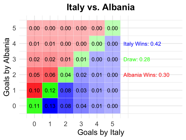
library(tidyverse)library(tidybayes)library(ggpubr)library(knitr)set.seed(42)# Function to calculate probabilities for a pairingcalculate_probabilities <-function(team1, team2, teams, hfit) {cat(sprintf('## %s vs %s\n', team1, team2)) id1 <-which(teams == team1) id2 <-which(teams == team2)# Spread draws and filter the relevant data As <- hfit %>% tidybayes::spread_draws(A[i, j]) %>%select(i, j, A) att_1 <- As %>%filter(j == id1, i ==1) att_2 <- As %>%filter(j == id2, i ==1) def_1 <- As %>%filter(j == id1, i ==2) def_2 <- As %>%filter(j == id2, i ==2) theta_1 <-exp(att_1$A - def_2$A) theta_2 <-exp(att_2$A - def_1$A)#g_1 <- rpois(length(theta_1), theta_1)#g_2 <- rpois(length(theta_2), theta_2)# Calculate probabilities#prob_win <- mean(g_1 > g_2)#prob_draw <- mean(g_1 == g_2)#prob_lose <- mean(g_1 < g_2) prob_g1=apply(matrix(0:10, ncol=1), 1, function(x) calc_prob(x, theta_1)) prob_g2=apply(matrix(0:10, ncol=1), 1, function(x) calc_prob(x, theta_2)) prob_goals =outer(prob_g1, prob_g2, '*') %>% as.matrix prob_draw =sum(diag(prob_goals)) prob_win =sum(prob_goals[lower.tri(prob_goals, diag =FALSE)]) prob_lose =sum(prob_goals[upper.tri(prob_goals, diag =FALSE)])# Return the probabilities and goalslist(prob_win =round(prob_win,2),prob_draw =round(prob_draw,2),prob_lose =round(prob_lose,2) )}### Group stage matches# Quite a pain to get the data in the right format from a lying ChatGPTlibrary(data.table)# Read the data from the CSVcsv_data <-"MatchNumber, Date, Team1, Team2, KickoffTime1, 14.06, Germany, Scotland, 21:002, 15.06, Hungary, Switzerland, 15:003, 15.06, Spain, Croatia, 18:004, 15.06, Italy, Albania, 21:005, 16.06, Poland, Netherlands, 15:006, 16.06, Slovenia, Denmark, 18:007, 16.06, Serbia, England, 21:008, 17.06, Romania, Ukraine, 15:009, 17.06, Belgium, Slovakia, 18:0010, 17.06, Austria, France, 21:0011, 18.06, Türkiye, Georgia, 15:0012, 18.06, Portugal, Czechia, 18:0013, 19.06, Croatia, Albania, 15:0014, 19.06, Germany, Hungary, 18:0015, 19.06, Scotland, Switzerland, 21:0016, 19.06, Spain, Italy, 21:0017, 20.06, Slovenia, Serbia, 15:0018, 20.06, Denmark, England, 18:0019, 20.06, Poland, Austria, 15:0020, 20.06, Netherlands, France, 21:0021, 21.06, Slovakia, Ukraine, 15:0022, 21.06, Belgium, Romania, 18:0023, 21.06, Türkiye, Portugal, 21:0024, 21.06, Georgia, Czechia, 18:0025, 23.06, Switzerland, Germany, 21:0026, 23.06, Scotland, Hungary, 21:0027, 24.06, Croatia, Italy, 21:0028, 24.06, Albania, Spain, 21:0029, 25.06, Netherlands, Austria, 18:0030, 25.06, France, Poland, 18:0031, 25.06, England, Slovenia, 21:0032, 25.06, Denmark, Serbia, 21:0033, 26.06, Slovakia, Romania, 18:0034, 26.06, Ukraine, Belgium, 18:0035, 26.06, Czechia, Türkiye, 21:0036, 26.06, Georgia, Portugal, 21:00"# Convert CSV data to data tablematches_raw <-fread(text = csv_data)matches =data.frame(Date=as.Date(paste0('2024-06-', matches_raw$Date)), Time=paste0(matches_raw$KickoffTime, ' CEST'), HomeTeam=matches_raw$Team1, AwayTeam=matches_raw$Team2)results =data.frame(num=NULL,Date=NULL, Time=NULL, HomeTeam=NULL, AwayTeam=NULL, Win=NULL, Draw=NULL, Lose=NULL)for (i in1:nrow(matches)) {# i=1#cat(sprintf('## %s vs %s\n', matches[i,3], matches[i,4])) probs <-calculate_probabilities(matches[i,3,drop=TRUE], matches[i,4,drop=TRUE], teams, hfit)cat(sprintf('Win: %.2f, Draw: %.2f, Lose: %.2f\n', probs$prob_win, probs$prob_draw, probs$prob_lose)) results =rbind(results, data.frame(Number = i,Date=matches[i,1], Time=matches[i,2], HomeTeam=matches[i,3], AwayTeam=matches[i,4], Win=probs$prob_win, Draw=probs$prob_draw, Lose=probs$prob_lose))}## ## Germany vs Scotland## Win: 0.46, Draw: 0.26, Lose: 0.28## ## Hungary vs Switzerland## Win: 0.37, Draw: 0.27, Lose: 0.36## ## Spain vs Croatia## Win: 0.52, Draw: 0.23, Lose: 0.25## ## Italy vs Albania## Win: 0.42, Draw: 0.28, Lose: 0.30## ## Poland vs Netherlands## Win: 0.31, Draw: 0.26, Lose: 0.43## ## Slovenia vs Denmark## Win: 0.37, Draw: 0.27, Lose: 0.36## ## Serbia vs England## Win: 0.18, Draw: 0.24, Lose: 0.58## ## Romania vs Ukraine## Win: 0.44, Draw: 0.28, Lose: 0.28## ## Belgium vs Slovakia## Win: 0.51, Draw: 0.26, Lose: 0.23## ## Austria vs France## Win: 0.35, Draw: 0.24, Lose: 0.41## ## Türkiye vs Georgia## Win: 0.41, Draw: 0.26, Lose: 0.33## ## Portugal vs Czechia## Win: 0.44, Draw: 0.25, Lose: 0.31## ## Croatia vs Albania## Win: 0.37, Draw: 0.29, Lose: 0.35## ## Germany vs Hungary## Win: 0.40, Draw: 0.27, Lose: 0.33## ## Scotland vs Switzerland## Win: 0.32, Draw: 0.26, Lose: 0.42## ## Spain vs Italy## Win: 0.46, Draw: 0.23, Lose: 0.30## ## Slovenia vs Serbia## Win: 0.46, Draw: 0.27, Lose: 0.26## ## Denmark vs England## Win: 0.27, Draw: 0.25, Lose: 0.48## ## Poland vs Austria## Win: 0.27, Draw: 0.26, Lose: 0.47## ## Netherlands vs France## Win: 0.31, Draw: 0.23, Lose: 0.46## ## Slovakia vs Ukraine## Win: 0.36, Draw: 0.28, Lose: 0.36## ## Belgium vs Romania## Win: 0.43, Draw: 0.27, Lose: 0.30## ## Türkiye vs Portugal## Win: 0.24, Draw: 0.23, Lose: 0.53## ## Georgia vs Czechia## Win: 0.26, Draw: 0.27, Lose: 0.47## ## Switzerland vs Germany## Win: 0.33, Draw: 0.25, Lose: 0.42## ## Scotland vs Hungary## Win: 0.31, Draw: 0.28, Lose: 0.41## ## Croatia vs Italy## Win: 0.31, Draw: 0.27, Lose: 0.42## ## Albania vs Spain## Win: 0.24, Draw: 0.24, Lose: 0.52## ## Netherlands vs Austria## Win: 0.33, Draw: 0.24, Lose: 0.43## ## France vs Poland## Win: 0.51, Draw: 0.24, Lose: 0.25## ## England vs Slovenia## Win: 0.47, Draw: 0.26, Lose: 0.27## ## Denmark vs Serbia## Win: 0.47, Draw: 0.26, Lose: 0.27## ## Slovakia vs Romania## Win: 0.28, Draw: 0.28, Lose: 0.44## ## Ukraine vs Belgium## Win: 0.23, Draw: 0.26, Lose: 0.51## ## Czechia vs Türkiye## Win: 0.44, Draw: 0.27, Lose: 0.29## ## Georgia vs Portugal## Win: 0.21, Draw: 0.22, Lose: 0.57# Print the summary table with linkskable(results, caption ="Probabilities of Match Outcomes", escape =FALSE)
Probabilities of Match Outcomes
Number
Date
Time
HomeTeam
AwayTeam
Win
Draw
Lose
1
2024-06-14
21:00 CEST
Germany
Scotland
0.46
0.26
0.28
2
2024-06-15
15:00 CEST
Hungary
Switzerland
0.37
0.27
0.36
3
2024-06-15
18:00 CEST
Spain
Croatia
0.52
0.23
0.25
4
2024-06-15
21:00 CEST
Italy
Albania
0.42
0.28
0.30
5
2024-06-16
15:00 CEST
Poland
Netherlands
0.31
0.26
0.43
6
2024-06-16
18:00 CEST
Slovenia
Denmark
0.37
0.27
0.36
7
2024-06-16
21:00 CEST
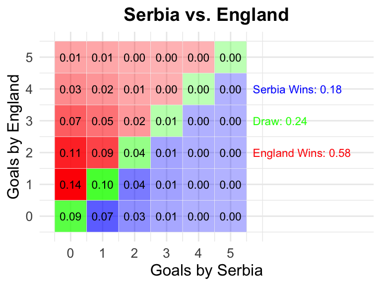
Serbia
England
0.18
0.24
0.58
8
2024-06-17
15:00 CEST
Romania
Ukraine
0.44
0.28
0.28
9
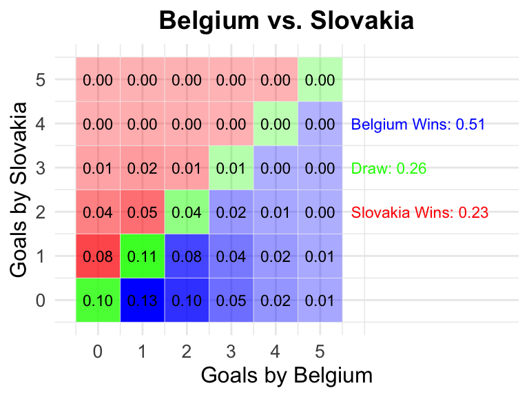
2024-06-17
18:00 CEST
Belgium
Slovakia
0.51
0.26
0.23
10
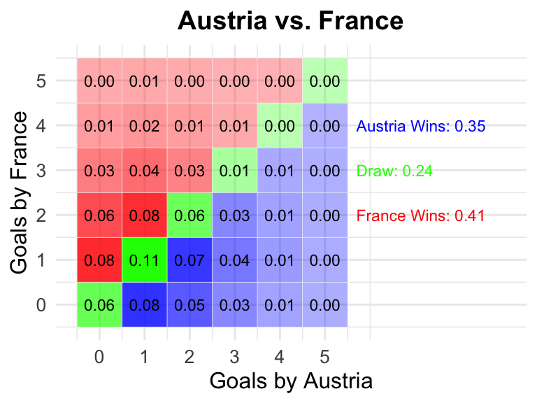
2024-06-17
21:00 CEST
Austria
France
0.35
0.24
0.41
11
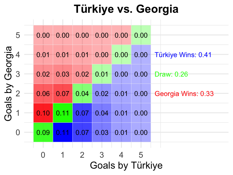
2024-06-18
15:00 CEST
Türkiye
Georgia
0.41
0.26
0.33
12
2024-06-18
18:00 CEST
Portugal
Czechia
0.44
0.25
0.31
13
2024-06-19
15:00 CEST
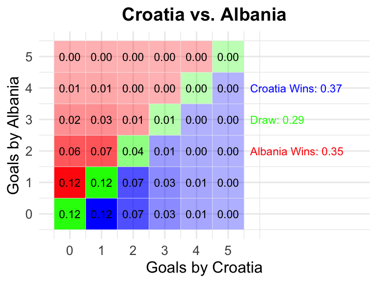
Croatia
Albania
0.37
0.29
0.35
14
2024-06-19
18:00 CEST
Germany
Hungary
0.40
0.27
0.33
15
2024-06-19
21:00 CEST
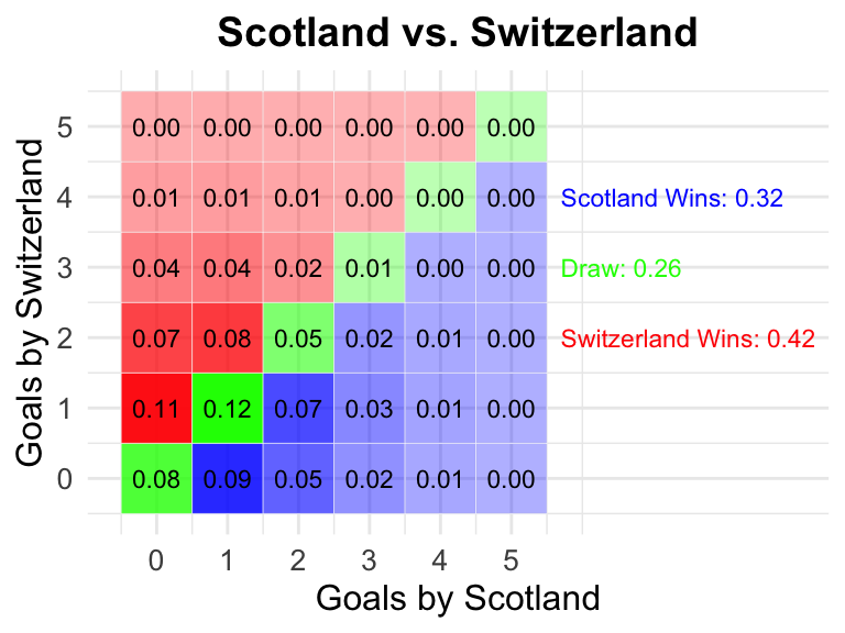
Scotland
Switzerland
0.32
0.26
0.42
16
2024-06-19
21:00 CEST
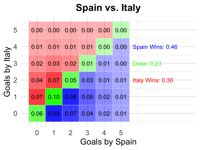
Spain
Italy
0.46
0.23
0.30
17
2024-06-20
15:00 CEST
Slovenia
Serbia
0.46
0.27
0.26
18
2024-06-20
18:00 CEST
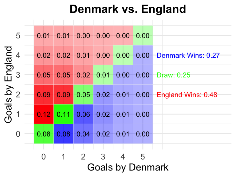
Denmark
England
0.27
0.25
0.48
19
2024-06-20
15:00 CEST
Poland
Austria
0.27
0.26
0.47
20
2024-06-20
21:00 CEST
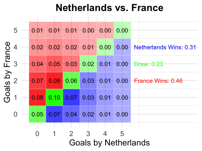
Netherlands
France
0.31
0.23
0.46
21
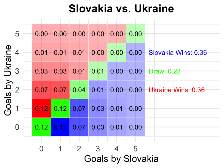
2024-06-21
15:00 CEST
Slovakia
Ukraine
0.36
0.28
0.36
22
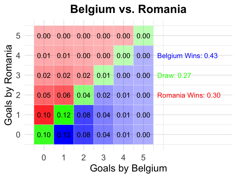
2024-06-21
18:00 CEST
Belgium
Romania
0.43
0.27
0.30
23
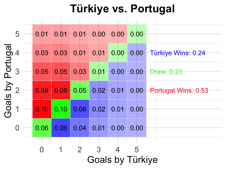
2024-06-21
21:00 CEST
Türkiye
Portugal
0.24
0.23
0.53
24
2024-06-21
18:00 CEST
Georgia
Czechia
0.26
0.27
0.47
25
2024-06-23
21:00 CEST
Switzerland
Germany
0.33
0.25
0.42
26
2024-06-23
21:00 CEST
Scotland
Hungary
0.31
0.28
0.41
27
2024-06-24
21:00 CEST
Croatia
Italy
0.31
0.27
0.42
28
2024-06-24
21:00 CEST
Albania
Spain
0.24
0.24
0.52
29
2024-06-25
18:00 CEST
Netherlands
Austria
0.33
0.24
0.43
30
2024-06-25
18:00 CEST
France
Poland
0.51
0.24
0.25
31
2024-06-25
21:00 CEST
England
Slovenia
0.47
0.26
0.27
32
2024-06-25
21:00 CEST
Denmark
Serbia
0.47
0.26
0.27
33
2024-06-26
18:00 CEST
Slovakia
Romania
0.28
0.28
0.44
34
2024-06-26
18:00 CEST
Ukraine
Belgium
0.23
0.26
0.51
35
2024-06-26
21:00 CEST
Czechia
Türkiye
0.44
0.27
0.29
36
2024-06-26
21:00 CEST
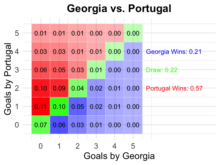
Georgia
Portugal
0.21
0.22
0.57
Details on individual games
Goal Distributions
1 Germany vs Scotland
2 Hungary vs Switzerland
3 Spain vs Croatia
4 Italy vs Albania
5 Poland vs Netherlands
6 Slovenia vs Denmark
7 Serbia vs England
8 Romania vs Ukraine
9 Belgium vs Slovakia
10 Austria vs France
11 Türkiye vs Georgia
12 Portugal vs Czechia
13 Croatia vs Albania
14 Germany vs Hungary
15 Scotland vs Switzerland
16 Spain vs Italy
17 Slovenia vs Serbia
18 Denmark vs England
19 Poland vs Austria
20 Netherlands vs France
21 Slovakia vs Ukraine
22 Belgium vs Romania
23 Türkiye vs Portugal
24 Georgia vs Czechia
25 Switzerland vs Germany
26 Scotland vs Hungary
27 Croatia vs Italy
28 Albania vs Spain
29 Netherlands vs Austria
30 France vs Poland
31 England vs Slovenia
32 Denmark vs Serbia
33 Slovakia vs Romania
34 Ukraine vs Belgium
35 Czechia vs Türkiye
36 Georgia vs Portugal
Source Code
---title: "Bayes is coming home - Predicting the Euro 2024 with Stan"author: "Oliver Dürr"format: html: toc: true toc-title: "Table of Contents" toc-depth: 3 fig-width: 6 fig-height: 3 code-fold: true code-tools: true mathjax: true # pdf: # toc: true # toc-title: "Table of Contents"filters: - webr---```{r, echo=FALSE, eval=TRUE, message=FALSE, warning=FALSE} library(tidyverse) library(kableExtra) set.seed(42)```<!--  -->The Euro 2024 ⚽ is a nice showcase of Bayesian Statistics. In Bayesian statistics, probabilities are seen as a degree of belief, which fits well with the nature of football. Almost everyone has beliefs about the strengths and weaknesses of the teams before seeing any games (based on historical data) and then updates these beliefs as new data comes in (games have been played).## Prediction based on the Historical DataWe load the matches prior to the Euro 2024, see <https://github.com/oduerr/da/blob/master/stan/Euro24/Euro_Data.md> how to get the data. Note the limitations of using historic; for example, Germany only started finding their form shortly before Euro 2024.## Loading the data```{r load_data, echo=FALSE, eval=TRUE, collapse=TRUE}# Uncomment the following line to read the data for the Euro 24data = read.csv('~/Documents/GitHub/da/stan/Euro24/games_before_euro24.csv', stringsAsFactors = FALSE)data = data[,1:4]colnames(data) = c('Home','score1', 'score2', 'Away')#kable(data[1:3,])```Loaded `r nrow(data)` games with `r length(unique(c(data$Home, data$Away)))` teams.::: {.callout-caution collapse="true"}## Expand To Learn How to set up the data for Stan## Preparing the data for Stan```{r preparing_for_stan}#Some R-Magic to convert the team names to numbers, no need to understand thisng = nrow(data)teams = unique(data$Home)nt = length(teams)ht = unlist(sapply(1:ng, function(g) which(teams == data$Home[g])))at = unlist(sapply(1:ng, function(g) which(teams == data$Away[g])))np=1 #Number games leaving out for predictionngob = ng-np #ngames obsered ngob = number of games to fit#print(paste0("Using the first ", ngob, " games to fit the model and ", np, " games to predict.", "Num teams ", length(teams)))my_data = list( nt = nt, ng = ngob, ht = ht[1:ngob], at = at[1:ngob], s1 = data$score1[1:ngob], s2 = data$score2[1:ngob], np = np, htnew = ht[(ngob+1):ng], atnew = at[(ngob+1):ng], s1new = data$score1[(ngob+1):ng], s2new = data$score2[(ngob+1):ng])```Using the first `r ngob` games to fit the model and `r np` games to predict. In total we have `r length(teams)` teams.:::## A Model for the goals scored 🥅We will assume that the number of goals scored by the home team $s_1$ and the away team $s_2$ follows a Poisson distribution. This has been shown to be a good model for the number of goals scored in a football match. We model the rate parameter $\theta$ of the Poisson distribution, related to the attack and defense strengths of the teams, as follows:$$ s_1 \sim \text{Pois}(\theta_1) \quad\text{goals scored by the home team}$$$$ s_2 \sim \text{Pois}(\theta_2) \quad\text{goals scored by the away team}$$ This is equivalent to performing two separate Poisson regressions, one for each team.We assume that:$$ \theta_1 = \exp(\text{home} + \text{att}_\text{ht} - \text{def}_\text{at})$$$$ \theta_2 = \exp(\text{att}_\text{at} - \text{def}_\text{ht})$$Since there is no home advantage in the Euro (except for Germany), we set $\text{home} = 0$.### Prior for the attack and defence strengthIn Bayesian statistics, we further need to specify a prior for the parameters (our degree of believe in the attack and defense abilities before seeing any data). For that we use a hierarchical model with correlated parameters. Other models are investigated at [comp_premier_league](comp_premier_league.html) for the English Premier League 2019/2020 season and for the German Bundesliga [2000](comp_bundes_liga_2000.html) and [2024](comp_bundes_liga.html) where the hierarchical model have been especially successful. The model is adopted from the [blog_post](https://github.com/MaggieLieu/STAN_tutorials/tree/master/Hierarchical) and the [paper](https://discovery.ucl.ac.uk/id/eprint/16040/1/16040.pdf). We extend the model to include a correlation between the attack and defense strength of the teams, since it is quite reasonable that a team that scores many goals (is above average in offense) is also good in defense.## Conditioning on the data / Fitting the modelAfter we state the model we fit the model to the data, or in Bayesian parlance, we update our degree of belief after seeing the data. ::: {.callout-caution collapse="true"}## Details of the model MCMC sampling with StanThe model is written in the probabilistic programming language Stan and can be found at <https://github.com/oduerr/da/blob/master/website/Euro24/hier_model_cor.stan>. This model used a Cholesky decomposition to model the correlation between the attack and defense strength of the teams. While this produces very effective sampling and is numerically stable, the Cholesky decomposition adds another layer of complexity to the model. We also provide a model without the Cholesky decomposition at <https://github.com/oduerr/da/blob/master/website/Euro24/hier_model_cor_nocholesky.stan> which is easier to understand but which is, besides the numerical difficulties, equivalent to the model with the Cholesky decomposition. ```{r, message=FALSE, collapse=TRUE, warning=FALSE, fig.width=10, fig.height=3}library(cmdstanr)options(mc.cores = parallel::detectCores())hmodel <- cmdstan_model('~/Documents/GitHub/da/website/Euro24/hier_model_cor.stan')#hmodel <- cmdstan_model('~/Documents/GitHub/da/website/Euro24/hier_model_cor_nocholsky.stan')hfit = hmodel$sample(data = my_data)p1 = bayesplot::mcmc_rhat_hist(bayesplot::rhat(hfit))p2 = bayesplot::mcmc_neff_hist(bayesplot::neff_ratio(hfit))ggpubr::ggarrange(p1, p2, ncol=2)```The fitting of the model is good, as the Rhat values are close to 1 and we have no divergent transitions. The effective sample size is also good. :::## The fitted modelWe plot the means of the attack and defense strengths of the teams. Shown are the mean values along with the 25% and 75% quantiles. There is considerable uncertainty in the strengths of the teams, but that’s the nature of the game.```{r, message=FALSE, collapse=TRUE, warning=FALSE, fig.width=7, fig.height=7}library(tidyverse)library(tidybayes)# Step 1: Gather draws and calculate summary statistics with credible intervalsd = hfit %>% tidybayes::gather_draws(A[i, j]) %>% group_by(i, j) %>% summarise( average_value = mean(.value), lower = quantile(.value, 0.25), # Lower bound upper = quantile(.value, 0.75), # Upper bound .groups = "drop" )# Step 2: Create a matrix of the average valuesA = xtabs(average_value ~ i + j, data = d)# Step 3: Plot the average valuesplot(A[1,], A[2,], pch=20, xlab='Attack', ylab='Defence', main='Attack vs Defence')# Step 4: Add team labelstext(A[1,], A[2,], labels=teams, cex=0.7, adj=c(-0.05, -0.8))# Step 5: Add error bars for 66% credibility intervals# Reshape data for plottingd_wide <- d %>% spread(key = j, value = average_value)d_lower <- d %>% spread(key = j, value = lower)d_upper <- d %>% spread(key = j, value = upper)# Convert to matrices for easier plottingA_lower <- xtabs(lower ~ i + j, data = d)A_upper <- xtabs(upper ~ i + j, data = d)# Plot vertical error barsarrows(A[1,], A_lower[2,], A[1,], A_upper[2,], angle=90, code=3, length=0.05, col="lightblue", alpha=0.5)# Plot horizontal error barsarrows(A_lower[1,], A[2,], A_upper[1,], A[2,], angle=90, code=3, length=0.05, col="lightblue")```::: {.callout-caution collapse="true"}## Detailed explanations for a single match Germany vs ScotlandThe opening game of Euro 2024 was Germany vs. Scotland. In the plots below, we show the posterior probabilities for the attack and defense strengths of the teams. ```{r, message=FALSE, collapse=TRUE, warning=FALSE, fig.width=7, fig.height=3}library(dplyr)library(tidyr)library(ggplot2)library(tidybayes)# Function to calculate probabilities for a pairingid1 <- which(teams == 'Germany')id2 <- which(teams == 'Scotland')# Extract posterior distributions for Attack and Defenseattack_germany <- hfit %>% tidybayes::spread_draws(A[i, j]) %>% filter(j == id1, i == 1) %>% select(A)attack_scotland <- hfit %>% tidybayes::spread_draws(A[i, j]) %>% filter(j == id2, i == 1) %>% select(A)defense_germany <- hfit %>% tidybayes::spread_draws(A[i, j]) %>% filter(j == id1, i == 2) %>% select(A)defense_scotland <- hfit %>% tidybayes::spread_draws(A[i, j]) %>% filter(j == id2, i == 2) %>% select(A)# Combine data into a tidy data frametidy_df <- bind_rows( attack_germany %>% mutate(Statistic = "Attack", Country = "Germany"), attack_scotland %>% mutate(Statistic = "Attack", Country = "Scotland"), defense_germany %>% mutate(Statistic = "Defense", Country = "Germany"), defense_scotland %>% mutate(Statistic = "Defense", Country = "Scotland"))# Include the mean values in the plotggplot(tidy_df, aes(x = A, fill = Country)) + geom_density(alpha = 0.5) + facet_wrap(~ Statistic, scales = "free") + labs(title = "Posterior Distributions of Attack and Defense Strengths", x = "Strength", y = "Density") + geom_vline(data = tidy_df %>% group_by(Statistic, Country) %>% summarise(mean_A = mean(A)), aes(xintercept = mean_A, color = Country), linetype = "dashed") + theme_minimal() ```### Making predictionsWe can now make predictions for the game Germany vs Scotland. Below are the first samples of the posterior distribution for the attack and defense strengths of germany and scotland.```{r, message=FALSE, collapse=TRUE, warning=FALSE, eval=TRUE}# Extract first five samples for demonstrationdf = data.frame(attack_germany = attack_germany$A, defense_germany = defense_germany$A, attack_scotland = attack_scotland$A, defense_scotland = defense_scotland$A) %>% head() knitr::kable(df)```We use the samples for posterior row by row to sample the number of goals for Germany and Scotland. We can use the samples to calculate the probability of a win, draw or loss for Germany.### Probabilities for win/draw/loss```{r, echo=TRUE, collapse=FALSE, warning=FALSE} set.seed(42) theta_germany = exp(attack_germany$A - defense_scotland$A) theta_scotland = exp(attack_scotland$A - defense_germany$A) g_germany = rpois(length(theta_germany), theta_germany) g_scotland = rpois(length(theta_scotland), theta_scotland) # Alternative way to calculate the probabilities calc_prob <- function(observed, theta) { mean(dpois(observed, theta)) } plot(table(g_germany)/length(g_germany), main='Germany Goals', xlab='Goals', ylab='Probability') prob_goals_germany = apply(matrix(0:10, ncol=1), 1, function(x) calc_prob(x, theta_germany)) points(0:5, prob_goals_germany[1:6]) prob_goals_scotland = apply(matrix(0:10, ncol=1), 1, function(x) calc_prob(x, theta_scotland)) plot(table(g_scotland)/length(g_scotland), main='Scotland Goals', xlab='Goals', ylab='Probability') points(0:5, prob_goals_scotland[1:6]) prob_goals = outer(prob_goals_germany, prob_goals_scotland, '*') sum(prob_goals) #Should be very close to 1 print(paste0('Germany wins (simu) ', mean(g_germany > g_scotland), #Probability of Germany winning ' probs', round(sum(prob_goals[lower.tri(prob_goals, diag = FALSE)]),4))) mean(g_germany < g_scotland) #Probability of Scotland winning mean(g_germany == g_scotland) #Probability of a draw print(paste0('Draw (simu) ', mean(g_germany == g_scotland), #Probability of a draw ' probs', sum(diag(prob_goals)))) print(paste0('Scotland wins (simu) ', mean(g_germany < g_scotland), #Probability of Germany winning ' probs', round(sum(prob_goals[upper.tri(prob_goals, diag = FALSE)]),4)))```Another way to look at is is at the joint distribution of the goals scored```{r goal_plot, echo=TRUE, collapse=FALSE, warning=FALSE, fig.width=4, fig.height=3}library(tidyverse)library(ggplot2)# Define the functionplot_goal_probabilities <- function(attack_team1, defense_team1, attack_team2, defense_team2, team1_name = "Team 1", team2_name = "Team 2") { set.seed(42) # Simulate goals scored using Poisson distribution theta_team1 <- exp(attack_team1 - defense_team2) theta_team2 <- exp(attack_team2 - defense_team1) #g_team1 <- rpois(length(theta_team1), theta_team1) #g_team2 <- rpois(length(theta_team2), theta_team2) # Calculate joint probabilities #joint_prob <- table(g_team1, g_team2) / length(g_team1) prob_g1= apply(matrix(0:10, ncol=1), 1, function(x) calc_prob(x, theta_team1)) prob_g2= apply(matrix(0:10, ncol=1), 1, function(x) calc_prob(x, theta_team2)) df_joint = outer(prob_g1, prob_g2, '*') %>% as.matrix df_joint <- reshape2::melt(df_joint, varnames = c("g_team1", "g_team2"), value.name = "Freq") #df_joint <- as.data.frame(as.table(joint_prob)) colnames(df_joint) <- c("Goals_Team1", "Goals_Team2", "Probability") df_joint$Goals_Team1 = df_joint$Goals_Team1 - 1 df_joint$Goals_Team2 = df_joint$Goals_Team2 - 1 # Ensure all combinations from 0 to 5 are included #all_combinations <- expand.grid(Goals_Team1 = 0:5, Goals_Team2 = 0:5) #df_joint <- merge(all_combinations, df_joint, by = c("Goals_Team1", "Goals_Team2"), all.x = TRUE) #df_joint$Probability[is.na(df_joint$Probability)] <- 0 # Calculate outcomes df_joint <- df_joint %>% mutate( Outcome = case_when( Goals_Team1 > Goals_Team2 ~ "Win1", Goals_Team1 < Goals_Team2 ~ "Win2", TRUE ~ "Draw" ) ) # Calculate probabilities prob_team1_win <- sum(df_joint$Probability[df_joint$Outcome == "Win1"]) prob_team2_win <- sum(df_joint$Probability[df_joint$Outcome == "Win2"]) prob_draw <- sum(df_joint$Probability[df_joint$Outcome == "Draw"]) # Print probabilities to the console # cat("Probability of", team1_name, "winning: ", prob_team1_win, "\n") # cat("Probability of", team2_name, "winning: ", prob_team2_win, "\n") # cat("Probability of a draw: ", prob_draw, "\n") # Plot the joint probabilities with labels and different colors for outcomes d = df_joint %>% filter(df_joint$Goals_Team1 <= 5) joint_plot <- ggplot(d, aes(x = Goals_Team1, y = Goals_Team2, fill = Outcome)) + geom_tile(color = "white", aes(alpha = Probability)) + geom_text(aes(label = sprintf("%.2f", Probability)), color = "black", size = 3) + scale_fill_manual(values = c("Win1" = "blue", "Win2" = "red", "Draw" = "green"), guide = NULL) + scale_alpha(range = c(0.3, 1), guide = NULL) + labs(title = paste0(team1_name, " vs. ", team2_name), x = paste("Goals by", team1_name), y = paste("Goals by", team2_name)) + theme_minimal() + theme( plot.title = element_text(hjust = 0.5, size = 14, face = "bold"), axis.title = element_text(size = 12), axis.text = element_text(size = 10) ) + scale_x_continuous(limits = c(-0.5, 9), breaks = 0:5) + scale_y_continuous(limits = c(-0.5, 5.5), breaks = 0:5) + annotate("text", x = 5.7, y = 4, label = sprintf("%s Wins: %.2f", team1_name, prob_team1_win), color = "blue", size = 3, hjust = 0) + annotate("text", x = 5.7, y = 3, label = sprintf("Draw: %.2f", prob_draw), color = "green", size = 3, hjust = 0) + annotate("text", x = 5.7, y = 2, label = sprintf("%s Wins: %.2f", team2_name, prob_team2_win), color = "red", size = 3, hjust = 0) # Print the joint plot return(joint_plot)}# Call the functionplot_goal_probabilities(attack_team1=attack_germany$A, defense_team1 = defense_germany$A, attack_team2=attack_scotland$A, defense_team2 = defense_scotland$A, team1_name="Germany", team2_name="Scotland")```Remember the result? It was 5:1 for Germany, so quite unexpected by the model. So that these predictions with a grain of salt. The model is based on historical data and does not take into account the current form of the teams.:::# Predictions::: callout-caution Note that these predictions are based on historical data and might do not take into account the current form of the teams. :::Note that there are some wrong dates in the list.```{r, message=FALSE, collapse=TRUE, warning=FALSE}library(tidyverse)library(tidybayes)library(ggpubr)library(knitr)set.seed(42)# Function to calculate probabilities for a pairingcalculate_probabilities <- function(team1, team2, teams, hfit) { cat(sprintf('## %s vs %s\n', team1, team2)) id1 <- which(teams == team1) id2 <- which(teams == team2) # Spread draws and filter the relevant data As <- hfit %>% tidybayes::spread_draws(A[i, j]) %>% select(i, j, A) att_1 <- As %>% filter(j == id1, i == 1) att_2 <- As %>% filter(j == id2, i == 1) def_1 <- As %>% filter(j == id1, i == 2) def_2 <- As %>% filter(j == id2, i == 2) theta_1 <- exp(att_1$A - def_2$A) theta_2 <- exp(att_2$A - def_1$A) #g_1 <- rpois(length(theta_1), theta_1) #g_2 <- rpois(length(theta_2), theta_2) # Calculate probabilities #prob_win <- mean(g_1 > g_2) #prob_draw <- mean(g_1 == g_2) #prob_lose <- mean(g_1 < g_2) prob_g1= apply(matrix(0:10, ncol=1), 1, function(x) calc_prob(x, theta_1)) prob_g2= apply(matrix(0:10, ncol=1), 1, function(x) calc_prob(x, theta_2)) prob_goals = outer(prob_g1, prob_g2, '*') %>% as.matrix prob_draw = sum(diag(prob_goals)) prob_win = sum(prob_goals[lower.tri(prob_goals, diag = FALSE)]) prob_lose = sum(prob_goals[upper.tri(prob_goals, diag = FALSE)]) # Return the probabilities and goals list( prob_win = round(prob_win,2), prob_draw = round(prob_draw,2), prob_lose = round(prob_lose,2) )}### Group stage matches# Quite a pain to get the data in the right format from a lying ChatGPTlibrary(data.table)# Read the data from the CSVcsv_data <- "MatchNumber, Date, Team1, Team2, KickoffTime1, 14.06, Germany, Scotland, 21:002, 15.06, Hungary, Switzerland, 15:003, 15.06, Spain, Croatia, 18:004, 15.06, Italy, Albania, 21:005, 16.06, Poland, Netherlands, 15:006, 16.06, Slovenia, Denmark, 18:007, 16.06, Serbia, England, 21:008, 17.06, Romania, Ukraine, 15:009, 17.06, Belgium, Slovakia, 18:0010, 17.06, Austria, France, 21:0011, 18.06, Türkiye, Georgia, 15:0012, 18.06, Portugal, Czechia, 18:0013, 19.06, Croatia, Albania, 15:0014, 19.06, Germany, Hungary, 18:0015, 19.06, Scotland, Switzerland, 21:0016, 19.06, Spain, Italy, 21:0017, 20.06, Slovenia, Serbia, 15:0018, 20.06, Denmark, England, 18:0019, 20.06, Poland, Austria, 15:0020, 20.06, Netherlands, France, 21:0021, 21.06, Slovakia, Ukraine, 15:0022, 21.06, Belgium, Romania, 18:0023, 21.06, Türkiye, Portugal, 21:0024, 21.06, Georgia, Czechia, 18:0025, 23.06, Switzerland, Germany, 21:0026, 23.06, Scotland, Hungary, 21:0027, 24.06, Croatia, Italy, 21:0028, 24.06, Albania, Spain, 21:0029, 25.06, Netherlands, Austria, 18:0030, 25.06, France, Poland, 18:0031, 25.06, England, Slovenia, 21:0032, 25.06, Denmark, Serbia, 21:0033, 26.06, Slovakia, Romania, 18:0034, 26.06, Ukraine, Belgium, 18:0035, 26.06, Czechia, Türkiye, 21:0036, 26.06, Georgia, Portugal, 21:00"# Convert CSV data to data tablematches_raw <- fread(text = csv_data)matches = data.frame(Date=as.Date(paste0('2024-06-', matches_raw$Date)), Time=paste0(matches_raw$KickoffTime, ' CEST'), HomeTeam=matches_raw$Team1, AwayTeam=matches_raw$Team2)results = data.frame(num=NULL,Date=NULL, Time=NULL, HomeTeam=NULL, AwayTeam=NULL, Win=NULL, Draw=NULL, Lose=NULL)for (i in 1:nrow(matches)) { # i=1 #cat(sprintf('## %s vs %s\n', matches[i,3], matches[i,4])) probs <- calculate_probabilities(matches[i,3,drop=TRUE], matches[i,4,drop=TRUE], teams, hfit) cat(sprintf('Win: %.2f, Draw: %.2f, Lose: %.2f\n', probs$prob_win, probs$prob_draw, probs$prob_lose)) results = rbind(results, data.frame( Number = i, Date=matches[i,1], Time=matches[i,2], HomeTeam=matches[i,3], AwayTeam=matches[i,4], Win=probs$prob_win, Draw=probs$prob_draw, Lose=probs$prob_lose))}# Print the summary table with linkskable(results, caption = "Probabilities of Match Outcomes", escape = FALSE)```## Details on individual games### Goal Distributions```{r individual_plots, echo=FALSE, results='asis', fig.width=4, fig.height=3, warning=FALSE, message=FALSE}# Function to generate plot for a pairinggenerate_plot <- function(team1, team2, teams, hfit) { #cat(team1, team2) id1 <- which(teams == team1) id2 <- which(teams == team2) # Spread draws and filter the relevant data As <- hfit %>% tidybayes::spread_draws(A[i, j]) %>% select(i, j, A) att_1 <- As %>% filter(j == id1, i == 1) att_2 <- As %>% filter(j == id2, i == 1) def_1 <- As %>% filter(j == id1, i == 2) def_2 <- As %>% filter(j == id2, i == 2) theta_1 <- exp(att_1$A - def_2$A) theta_2 <- exp(att_2$A - def_1$A) g_1 <- rpois(length(theta_1), theta_1) g_2 <- rpois(length(theta_2), theta_2) # Calculate mean goals mean_g1 <- mean(g_1) mean_g2 <- mean(g_2) # Create a data frame for the goal distributions goal_dist <- data.frame( goals = c(g_1, g_2), team = rep(c(team1, team2), each = length(g_1)) ) # Plot the goal distributions for each team with mean values p1 <- ggplot(goal_dist %>% filter(team == team1), aes(x = factor(goals))) + geom_bar(aes(y = after_stat(count) / sum(after_stat(count))), fill = "blue", color = "black", alpha = 0.7) + labs(title = paste("Goals for", team1, "(Expected:", round(mean_g1, 2), ")"), x = "Goals", y = "Probability") + theme_minimal() + geom_vline(xintercept = mean_g1, linetype = "dashed", color = "blue") p2 <- ggplot(goal_dist %>% filter(team == team2), aes(x = factor(goals))) + geom_bar(aes(y = after_stat(count) / sum(after_stat(count))), fill = "red", color = "black", alpha = 0.7) + labs(title = paste("Goals for", team2, "(Expected:", round(mean_g2, 2), ")"), x = "Goals", y = "Probability") + theme_minimal() + geom_vline(xintercept = mean_g2, linetype = "dashed", color = "red") # Arrange the plots side by side combined_plot <- ggarrange(p1, p2, ncol = 2, nrow = 1) return(combined_plot)}# Generate plots for all pairings and display themfor (i in 1:nrow(matches)) { team1_name = matches[i,3] team2_name = matches[i,4] cat(sprintf('\n## %d %s vs %s\n',i, team1_name, team2_name)) id1 <- which(teams == team1_name) id2 <- which(teams == team2_name) # Getting the posterior draws for the attack and defense strengths As <- hfit %>% tidybayes::spread_draws(A[i, j]) %>% select(i, j, A) att_1 <- As %>% filter(j == id1, i == 1) att_2 <- As %>% filter(j == id2, i == 1) def_1 <- As %>% filter(j == id1, i == 2) def_2 <- As %>% filter(j == id2, i == 2) plot = plot_goal_probabilities(att_1$A, def_1$A, att_2$A, def_2$A, team1_name, team2_name) #plot <- generate_plot(matches[i,3,drop=TRUE], matches[i,4,drop=TRUE], teams, hfit) print(plot) cat(sprintf('\n'))}```