df <-mutate(df, name =sub("^.*/", "", name)) df_raw =read.csv('~/Documents/GitHub/da/website/Euro24/premierleague2019.csv')head(df_raw) %>%kable()
Div
Date
Time
HomeTeam
AwayTeam
FTHG
FTAG
FTR
HTHG
HTAG
HTR
Referee
HS
AS
HST
AST
HF
AF
HC
AC
HY
AY
HR
AR
B365H
B365D
B365A
BWH
BWD
BWA
IWH
IWD
IWA
PSH
PSD
PSA
WHH
WHD
WHA
VCH
VCD
VCA
MaxH
MaxD
MaxA
AvgH
AvgD
AvgA
B365.2.5
B365.2.5.1
P.2.5
P.2.5.1
Max.2.5
Max.2.5.1
Avg.2.5
Avg.2.5.1
AHh
B365AHH
B365AHA
PAHH
PAHA
MaxAHH
MaxAHA
AvgAHH
AvgAHA
B365CH
B365CD
B365CA
BWCH
BWCD
BWCA
IWCH
IWCD
IWCA
PSCH
PSCD
PSCA
WHCH
WHCD
WHCA
VCCH
VCCD
VCCA
MaxCH
MaxCD
MaxCA
AvgCH
AvgCD
AvgCA
B365C.2.5
B365C.2.5.1
PC.2.5
PC.2.5.1
MaxC.2.5
MaxC.2.5.1
AvgC.2.5
AvgC.2.5.1
AHCh
B365CAHH
B365CAHA
PCAHH
PCAHA
MaxCAHH
MaxCAHA
AvgCAHH
AvgCAHA
E0
09/08/2019
20:00
Liverpool
Norwich
4
1
H
4
0
H
M Oliver
15
12
7
5
9
9
11
2
0
2
0
0
1.14
10.00
19.00
1.14
8.25
18.50
1.15
8.00
18.00
1.15
9.59
18.05
1.12
8.5
21.00
1.14
9.5
23.00
1.16
10.00
23.00
1.14
8.75
19.83
1.40
3.00
1.40
3.11
1.45
3.11
1.41
2.92
-2.25
1.96
1.94
1.97
1.95
1.97
2.00
1.94
1.94
1.14
9.50
21.00
1.14
9.0
20.00
1.15
8.00
18.00
1.14
10.43
19.63
1.11
9.50
21.00
1.14
9.50
23.00
1.16
10.50
23.00
1.14
9.52
19.18
1.3
3.50
1.34
3.44
1.36
3.76
1.32
3.43
-2.25
1.91
1.99
1.94
1.98
1.99
2.07
1.90
1.99
E0
10/08/2019
12:30
West Ham
Man City
0
5
A
0
1
A
M Dean
5
14
3
9
6
13
1
1
2
2
0
0
12.00
6.50
1.22
11.50
5.75
1.26
11.00
6.10
1.25
11.68
6.53
1.26
13.00
6.0
1.24
12.00
6.5
1.25
13.00
6.75
1.29
11.84
6.28
1.25
1.44
2.75
1.49
2.77
1.51
2.77
1.48
2.65
1.75
2.00
1.90
2.02
1.90
2.02
1.92
1.99
1.89
12.00
7.00
1.25
11.00
6.0
1.26
11.00
6.10
1.25
11.11
6.68
1.27
11.00
6.50
1.24
12.00
6.50
1.25
13.00
7.00
1.29
11.14
6.46
1.26
1.4
3.00
1.43
3.03
1.50
3.22
1.41
2.91
1.75
1.95
1.95
1.96
1.97
2.07
1.98
1.97
1.92
E0
10/08/2019
15:00
Bournemouth
Sheffield United
1
1
D
0
0
D
K Friend
13
8
3
3
10
19
3
4
2
1
0
0
1.95
3.60
3.60
1.95
3.60
3.90
1.97
3.55
3.80
2.04
3.57
3.90
2.00
3.5
3.80
2.00
3.6
4.00
2.06
3.65
4.00
2.01
3.53
3.83
1.90
1.90
1.96
1.96
2.00
1.99
1.90
1.93
-0.50
2.01
1.89
2.04
1.88
2.04
1.91
2.00
1.88
1.95
3.70
4.20
1.95
3.6
3.90
1.97
3.55
3.85
1.98
3.67
4.06
1.95
3.60
3.90
2.00
3.60
4.00
2.03
3.70
4.20
1.98
3.58
3.96
1.9
1.90
1.94
1.97
1.97
1.98
1.91
1.92
-0.50
1.95
1.95
1.98
1.95
2.00
1.96
1.96
1.92
E0
10/08/2019
15:00
Burnley
Southampton
3
0
H
0
0
D
G Scott
10
11
4
3
6
12
2
7
0
0
0
0
2.62
3.20
2.75
2.65
3.20
2.75
2.65
3.20
2.75
2.71
3.31
2.81
2.70
3.2
2.75
2.70
3.3
2.80
2.80
3.33
2.85
2.68
3.22
2.78
2.10
1.72
2.17
1.77
2.20
1.78
2.12
1.73
0.00
1.92
1.98
1.93
2.00
1.94
2.00
1.91
1.98
2.70
3.25
2.90
2.65
3.1
2.85
2.60
3.20
2.85
2.71
3.19
2.90
2.62
3.20
2.80
2.70
3.25
2.90
2.72
3.26
2.95
2.65
3.18
2.88
2.1
1.72
2.19
1.76
2.25
1.78
2.17
1.71
0.00
1.87
2.03
1.89
2.03
1.90
2.07
1.86
2.02
E0
10/08/2019
15:00
Crystal Palace
Everton
0
0
D
0
0
D
J Moss
6
10
2
3
16
14
6
2
2
1
0
1
3.00
3.25
2.37
3.20
3.20
2.35
3.10
3.20
2.40
3.21
3.37
2.39
3.10
3.3
2.35
3.20
3.3
2.45
3.21
3.40
2.52
3.13
3.27
2.40
2.20
1.66
2.23
1.74
2.25
1.74
2.18
1.70
0.25
1.85
2.05
1.88
2.05
1.88
2.09
1.84
2.04
3.40
3.50
2.25
3.30
3.3
2.25
3.40
3.30
2.20
3.37
3.45
2.27
3.30
3.30
2.25
3.40
3.30
2.25
3.55
3.50
2.34
3.41
3.37
2.23
2.2
1.66
2.22
1.74
2.28
1.77
2.17
1.71
0.25
1.82
2.08
1.97
1.96
2.03
2.08
1.96
1.93
E0
10/08/2019
15:00
Watford
Brighton
0
3
A
0
1
A
C Pawson
11
5
3
3
15
11
5
2
0
1
0
0
1.90
3.40
4.00
1.90
3.40
4.33
1.93
3.40
4.25
1.98
3.44
4.37
1.95
3.4
4.20
1.95
3.5
4.33
2.00
3.50
4.60
1.94
3.41
4.26
2.10
1.72
2.19
1.76
2.24
1.76
2.16
1.71
-0.50
1.95
1.95
1.98
1.95
1.98
1.98
1.94
1.94
2.10
3.25
4.20
2.10
3.1
4.00
2.05
3.20
4.00
2.05
3.38
4.12
2.05
3.25
4.00
2.15
3.30
3.90
2.15
3.38
4.20
2.07
3.27
4.04
2.1
1.72
2.16
1.78
2.20
1.78
2.14
1.73
-0.50
2.04
1.86
2.05
1.88
2.12
1.91
2.05
1.84
Model Comparisons
Code
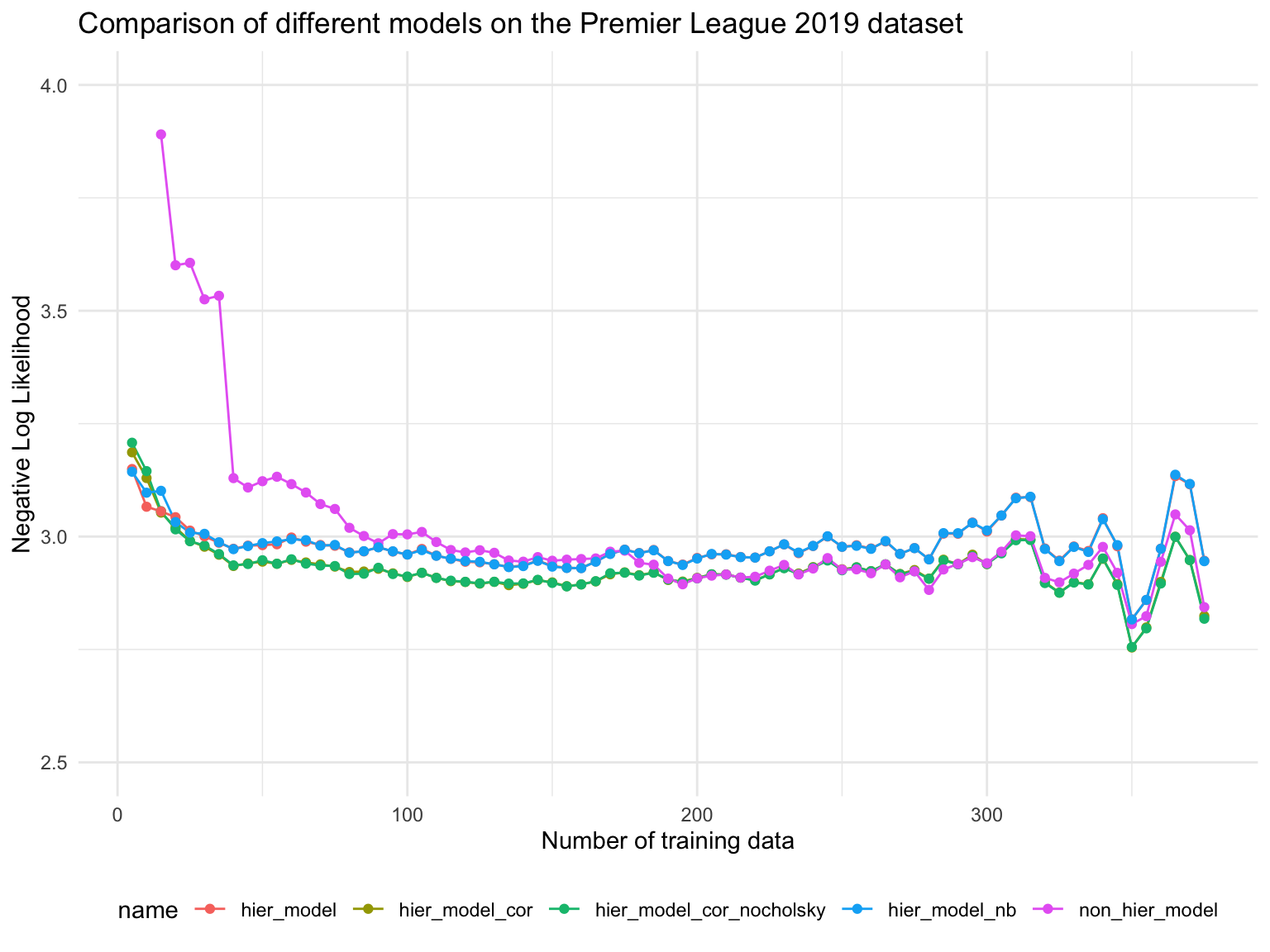
# Assuming df is your dataframe df %>%filter(type =='NLL_PRED') %>%ggplot(aes(x = ntrain, y = res, color = name)) +geom_line() +geom_point() +theme_minimal() +labs(title ='Comparison of different models on the Premier League 2019 dataset', x ='Number of training data', y ='Negative Log Likelihood' ) +ylim(2.5, 4) +theme(legend.position ="bottom") +coord_cartesian(clip ="off") # Allow lines to go outside the plot area
Observations
Especially for small training data, the hierarchical model performs better than the non-hierarchical model.
The Correlated Dataset model performs slightly better than non-correlated one
There is partically no difference in predictive performance when comparing the model with and without Cholesky decomposition.
The negative binomial model performs comparable to Poisson model.
All models start to deteriorate at around 280 training data. This is due to the interruped season in 2019/2020 due to the COVID-19 pandemic.
Comparison of predicted vs PSIS-LOO
Code
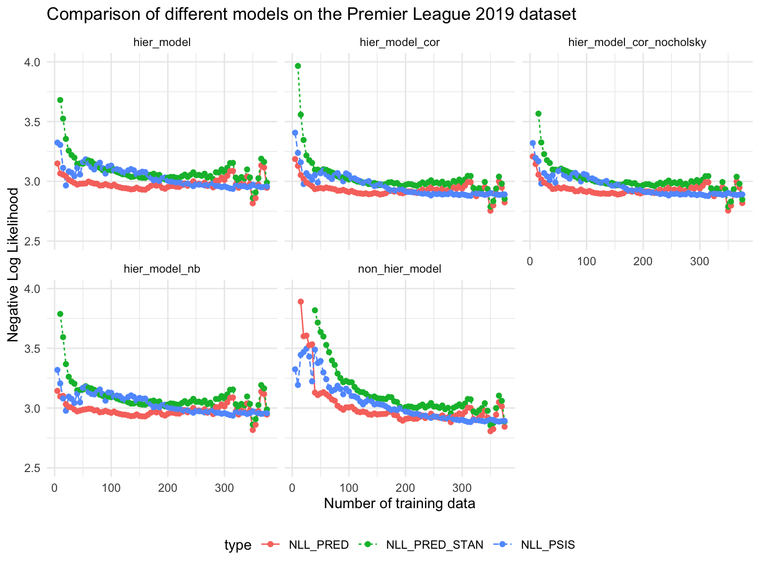
df %>%filter(type %in%c('NLL_PRED', 'NLL_PSIS', 'NLL_PRED_STAN')) %>%ggplot(aes(x = ntrain, y = res, color = type)) +geom_line(aes(linetype = type)) +geom_point() +theme_minimal() +labs(title ='Comparison of different models on the Premier League 2019 dataset', x ='Number of training data', y ='Negative Log Likelihood' ) +ylim(2.5, 4) +facet_wrap(~name) +theme(legend.position ="bottom") +coord_cartesian(clip ="off") # Allow lines to go outside the plot area
Observations
For few training data, PSIS-LOO estimator is
Result NLLs
Code
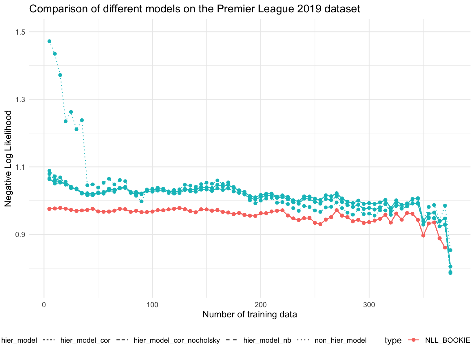
df %>%filter(type %in%c('NLL_RESULTS', 'NLL_BOOKIE')) %>%ggplot(aes(x = ntrain, y = res, color = type)) +geom_line(aes(linetype = name)) +geom_point() +theme_minimal() +labs(title ='Comparison of different models on the Premier League 2019 dataset', x ='Number of training data', y ='Negative Log Likelihood' ) +ylim(0.75, 1.5) +theme(legend.position ="bottom") +coord_cartesian(clip ="off") # Allow lines to go outside the plot area
Betting Returns
Code
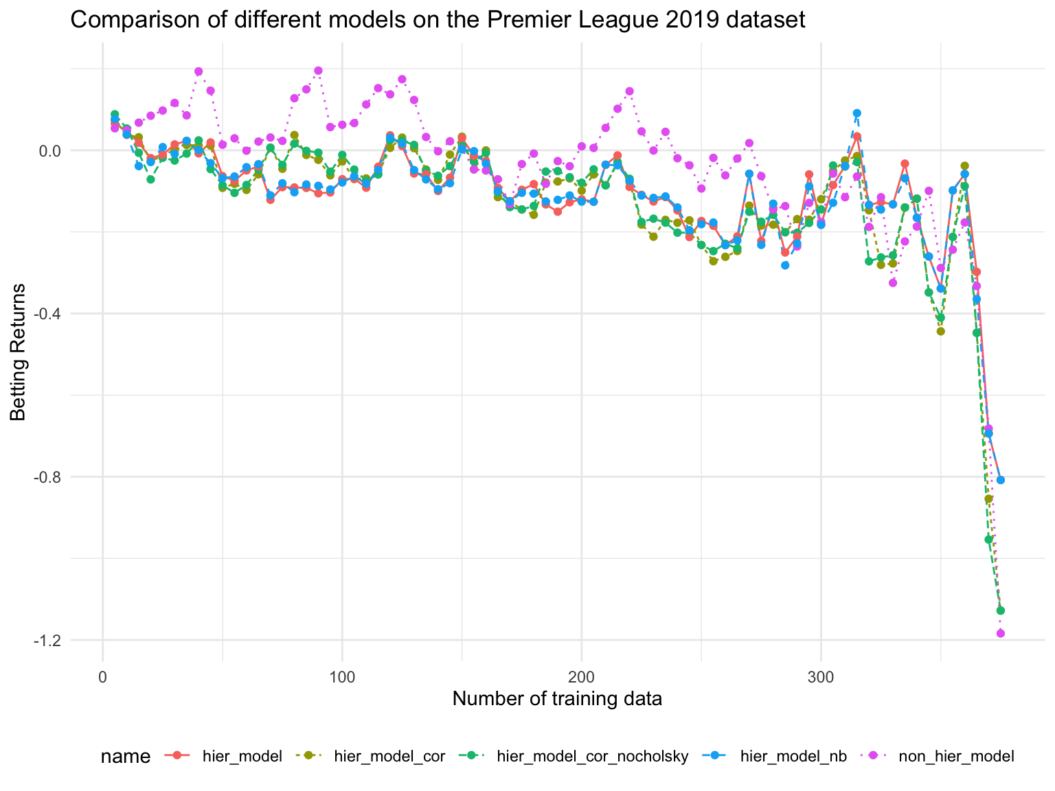
df %>%filter(type %in%c('BET_RETURN')) %>%ggplot(aes(x = ntrain, y = res, color = name)) +geom_line(aes(linetype = name)) +geom_point() +theme_minimal() +labs(title ='Comparison of different models on the Premier League 2019 dataset', x ='Number of training data', y ='Betting Returns' ) +#ylim(0.75, 1.5) +theme(legend.position ="bottom") +coord_cartesian(clip ="off") # Allow lines to go outside the plot area
Technical Details
Code
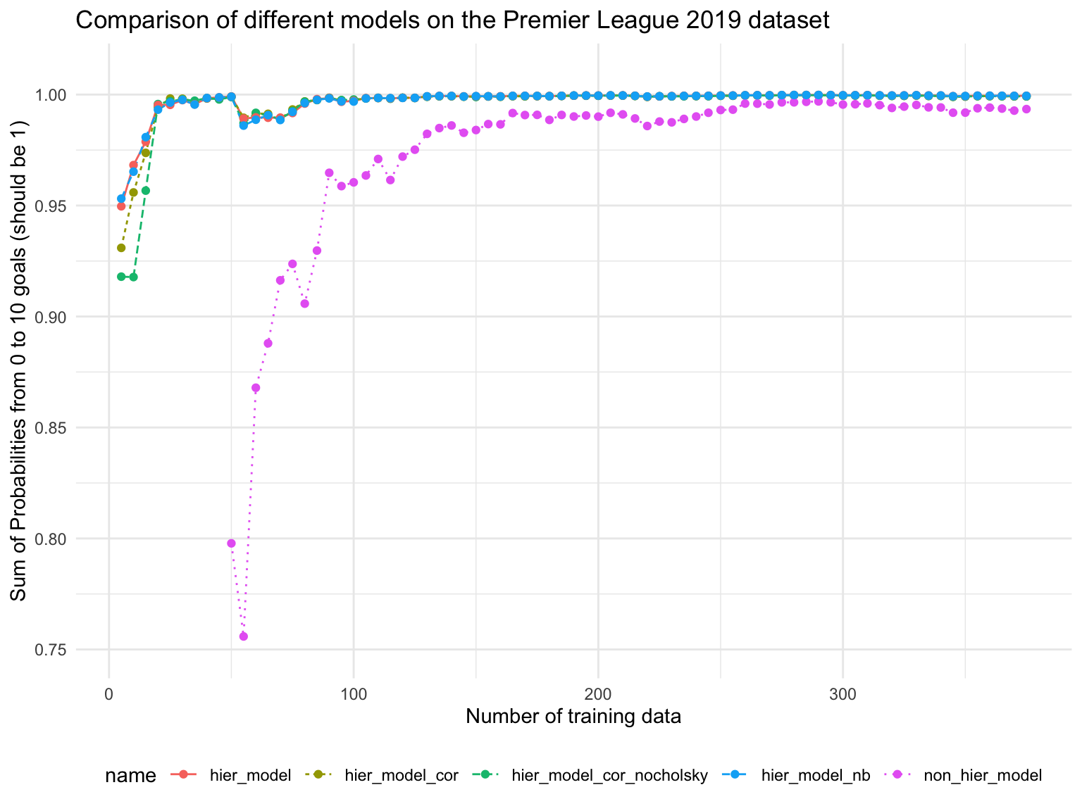
df %>%filter(type %in%c('MIN_SUM_PROB')) %>%ggplot(aes(x = ntrain, y = res, color = name)) +geom_line(aes(linetype = name)) +geom_point() +theme_minimal() +labs(title ='Comparison of different models on the Premier League 2019 dataset', x ='Number of training data', y ='Sum of Probabilities from 0 to 10 goals (should be 1)' ) +ylim(0.75, 1.01) +theme(legend.position ="bottom") +coord_cartesian(clip ="off") # Allow lines to go outside the plot area
Source Code
---title: "Comparison of different models on the Premier League 2019 dataset"author: "Oliver Dürr"format: html: toc: true toc-title: "Table of Contents" toc-depth: 3 fig-width: 6 fig-height: 3 code-fold: true code-tools: true mathjax: true # pdf: # toc: true # toc-title: "Table of Contents" # filters: #- webr---```{r, echo=FALSE, eval=TRUE, message=FALSE, warning=FALSE} library(tidyverse) library(kableExtra) set.seed(42)```The experiments take some time to run, therefore we used the R-Script to producte the results <https://github.com/oduerr/da/blob/master/website/Euro24/eval_performance_runner.R>.## Loading the data```{r, asis=TRUE} df = read.csv('~/Documents/GitHub/da/website/Euro24/eval_performance_premier_league_2019.csv') df %>% tail() %>% kable() df <- mutate(df, name = sub("^.*/", "", name)) df_raw = read.csv('~/Documents/GitHub/da/website/Euro24/premierleague2019.csv') head(df_raw) %>% kable()```## Model Comparisons```{r hier-vs-non, fig.width=8, fig.height=6, warning=FALSE, message=FALSE} # Assuming df is your dataframe df %>% filter(type == 'NLL_PRED') %>% ggplot(aes(x = ntrain, y = res, color = name)) + geom_line() + geom_point() + theme_minimal() + labs( title = 'Comparison of different models on the Premier League 2019 dataset', x = 'Number of training data', y = 'Negative Log Likelihood' ) + ylim(2.5, 4) + theme(legend.position = "bottom") + coord_cartesian(clip = "off") # Allow lines to go outside the plot area```### Observations- Especially for small training data, the hierarchical model performs better than the non-hierarchical model. - The Correlated Dataset model performs slightly better than non-correlated one- There is partically no difference in predictive performance when comparing the model with and without Cholesky decomposition. - The negative binomial model performs comparable to Poisson model.- All models start to deteriorate at around 280 training data. This is due to the interruped season in 2019/2020 due to the COVID-19 pandemic.## Comparison of predicted vs PSIS-LOO```{r pred-vs-loo, fig.width=8, fig.height=6, warning=FALSE, message=FALSE} df %>% filter(type %in% c('NLL_PRED', 'NLL_PSIS', 'NLL_PRED_STAN')) %>% ggplot(aes(x = ntrain, y = res, color = type)) + geom_line(aes(linetype = type)) + geom_point() + theme_minimal() + labs( title = 'Comparison of different models on the Premier League 2019 dataset', x = 'Number of training data', y = 'Negative Log Likelihood' ) + ylim(2.5, 4) + facet_wrap(~name) + theme(legend.position = "bottom") + coord_cartesian(clip = "off") # Allow lines to go outside the plot area```### Observations- For few training data, PSIS-LOO estimator is ## Result NLLs```{r nll, fig.width=8, fig.height=6, warning=FALSE, message=FALSE} df %>% filter(type %in% c('NLL_RESULTS', 'NLL_BOOKIE')) %>% ggplot(aes(x = ntrain, y = res, color = type)) + geom_line(aes(linetype = name)) + geom_point() + theme_minimal() + labs( title = 'Comparison of different models on the Premier League 2019 dataset', x = 'Number of training data', y = 'Negative Log Likelihood' ) + ylim(0.75, 1.5) + theme(legend.position = "bottom") + coord_cartesian(clip = "off") # Allow lines to go outside the plot area```## Betting Returns```{r betting, fig.width=8, fig.height=6, warning=FALSE, message=FALSE} df %>% filter(type %in% c('BET_RETURN')) %>% ggplot(aes(x = ntrain, y = res, color = name)) + geom_line(aes(linetype = name)) + geom_point() + theme_minimal() + labs( title = 'Comparison of different models on the Premier League 2019 dataset', x = 'Number of training data', y = 'Betting Returns' ) + #ylim(0.75, 1.5) + theme(legend.position = "bottom") + coord_cartesian(clip = "off") # Allow lines to go outside the plot area```## Technical Details```{r details, fig.width=8, fig.height=6, warning=FALSE, message=FALSE} df %>% filter(type %in% c('MIN_SUM_PROB')) %>% ggplot(aes(x = ntrain, y = res, color = name)) + geom_line(aes(linetype = name)) + geom_point() + theme_minimal() + labs( title = 'Comparison of different models on the Premier League 2019 dataset', x = 'Number of training data', y = 'Sum of Probabilities from 0 to 10 goals (should be 1)' ) + ylim(0.75, 1.01) + theme(legend.position = "bottom") + coord_cartesian(clip = "off") # Allow lines to go outside the plot area```